20180036 권혁태
Part1: Bias and Variance
Step 2-1: Polynomial Regression
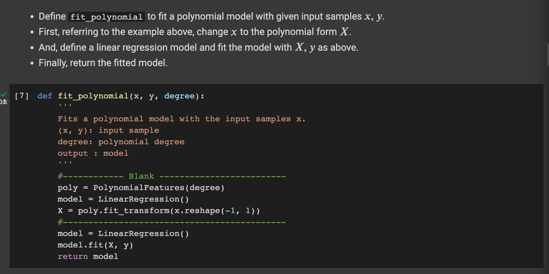
The fit_polynomial function takes in input samples x and y, and the degree of the polynomial degree to fit. what the y means is that the target data for training.
PolynomialFeatures from scikit-learn transforms the input feature x into a higher degree polynomial feature space. for example, the input x transforms into below forms
Then, it uses LinearRegression to fit a linear model to feature space. Finally, it returns the fitted model.
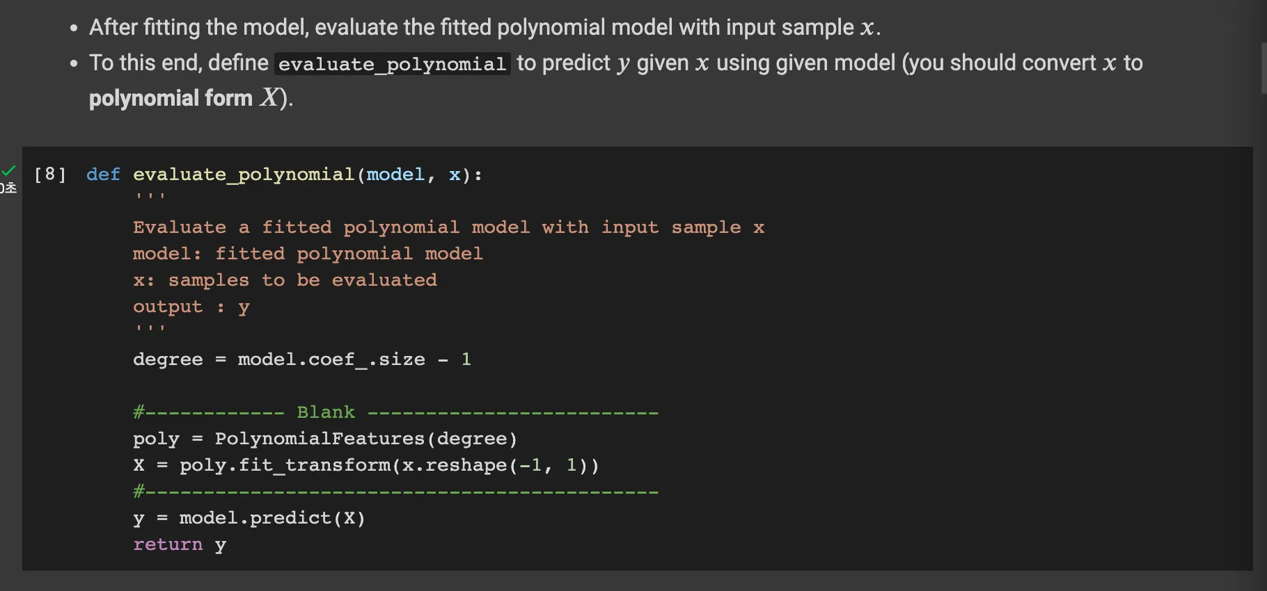
The evaluate_polynomial function takes in a fitted polynomial model model and an input sample x.
as the model has n+1 coefficients when the degree is n because of the bias. After this, it transforms the input feature x into a higher degree space using the PolynomialFeatures. Finally, it return predict output y.
Result
degree: 3
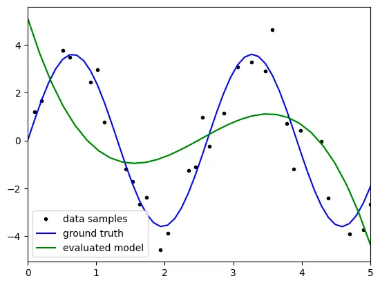
the above result is not satisfatory because it reveals big bias with
the new text sets.
the results might come from the 'underfitting' because the model
is not complex enough to predict the test data.
as the degree is 3, the terms the model can represent is
limited to degree 3, which is the second term of taylor series.
therefore, to get statisfactory result, we have to raise the degree up
Plain Text
복사
degree: 5
degree: 10
degree: 20
However, when the degree reaches 20, the graph seems like 'overFitting'
especially, the right section of graph seems like linearly even
the model is polynomial.
Plain Text
복사
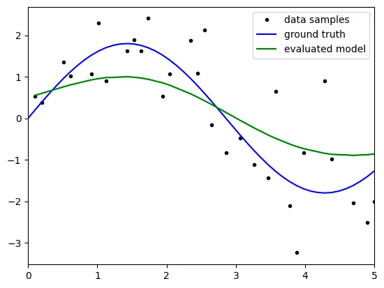
Step 2-2: Regression with Gaussian basis
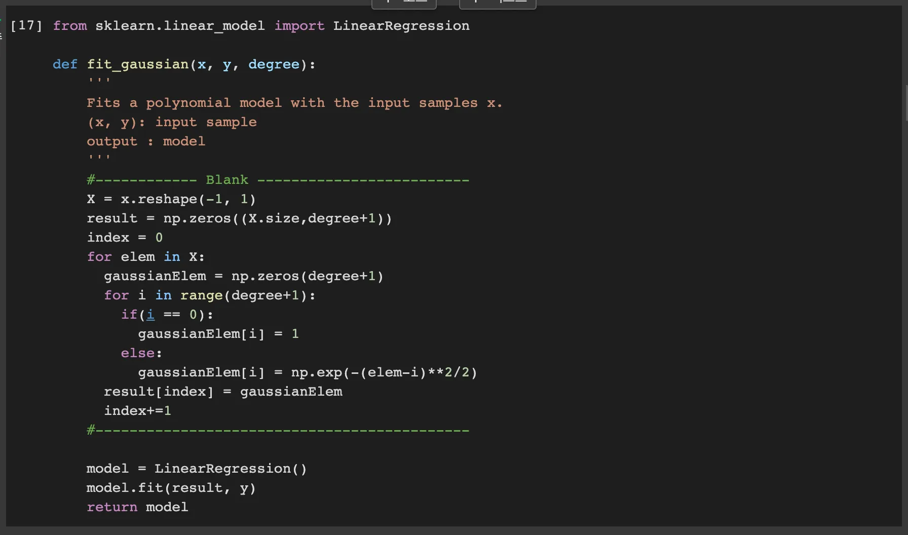
The fit_gaussian takes in three arguments. x, y, and degree. x and y are input samples, and degree determines the transformed vector space with gaussian function.
The function first transforms the input x into a higher degree space using Gaussian function. as the instruction said that for jth degree vector should have the mean as j. Therefore, using for-loop, compute the Gaussian basis function and fits the linear model to the transformed space.
it returns the fitted model
evaluate_gaussian takes in linear regression model which is fitted using the gaussian as basis function.
Same as polynomial regression, the degree is the number of model’s coefficient subtracted by 1 because the model contains the bias 1.
After this, the function initializes an array result with zeros for storing the computed Gaussian basis functions, and compute and transforme the input into higher degree space with Gaussian function as the models did.
Finally, the function returns the predicted output y
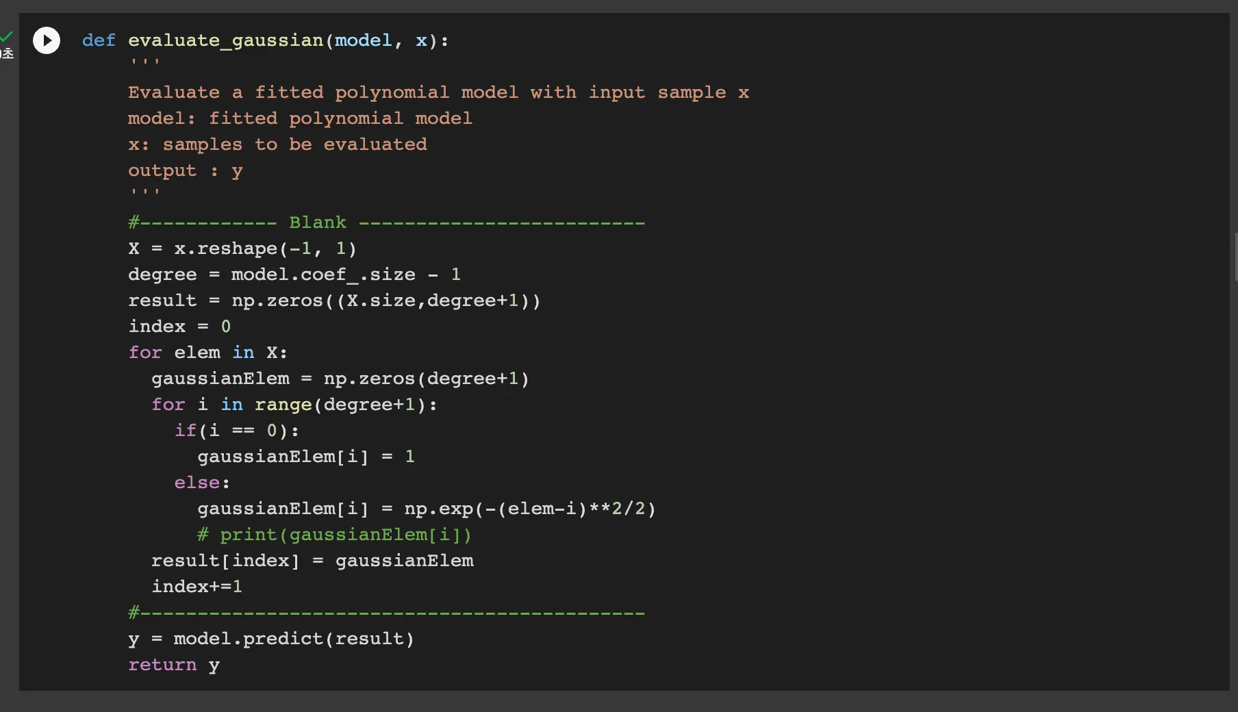
Result
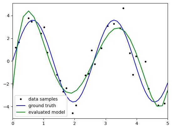
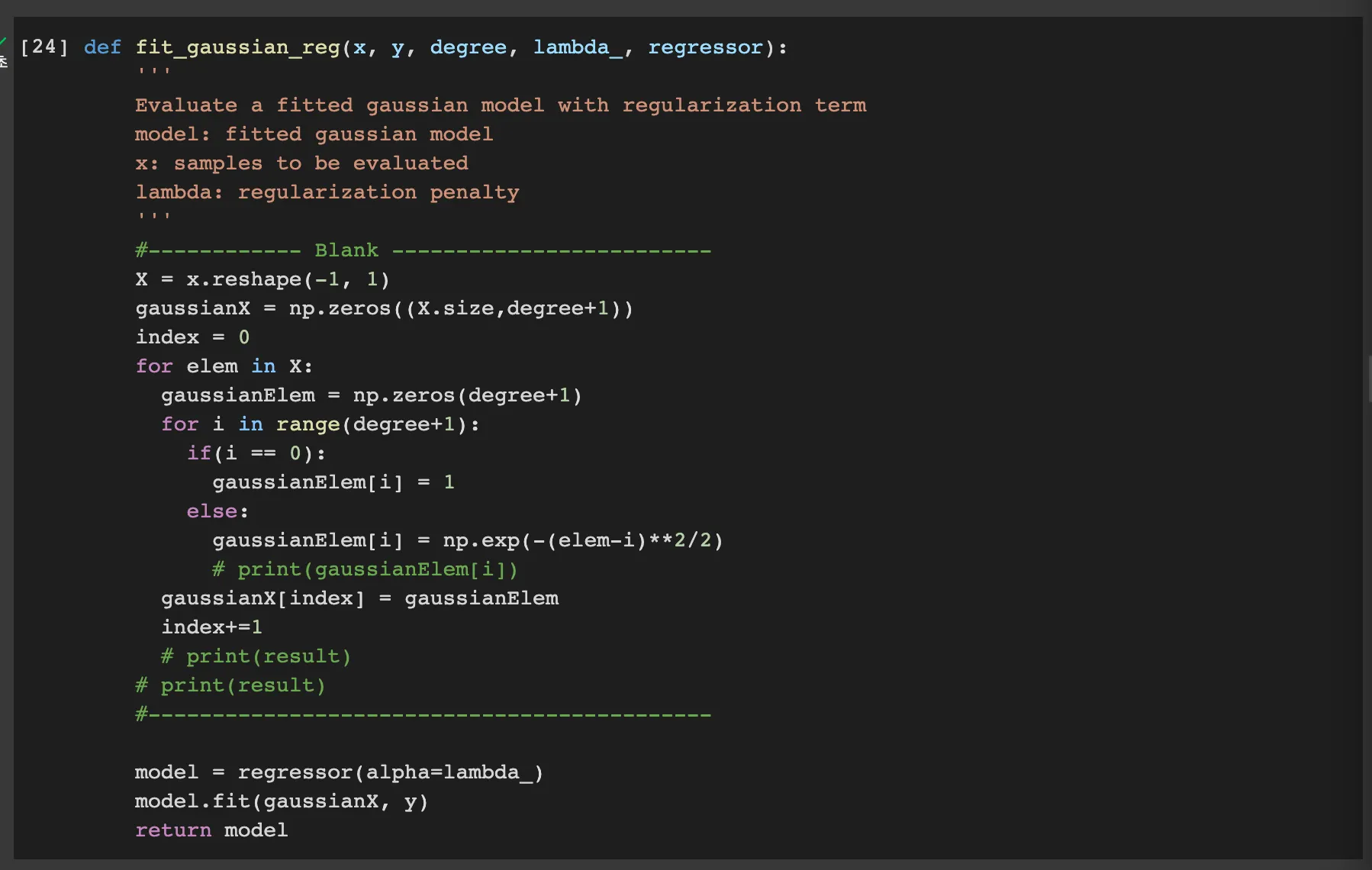
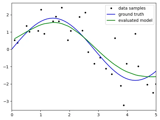
degree: 10
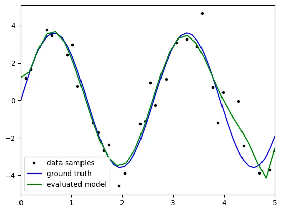
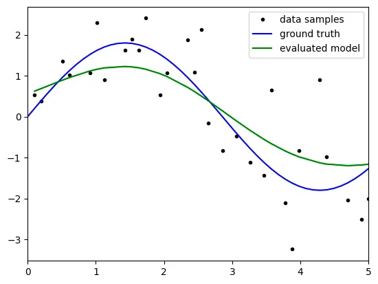
degree: 5
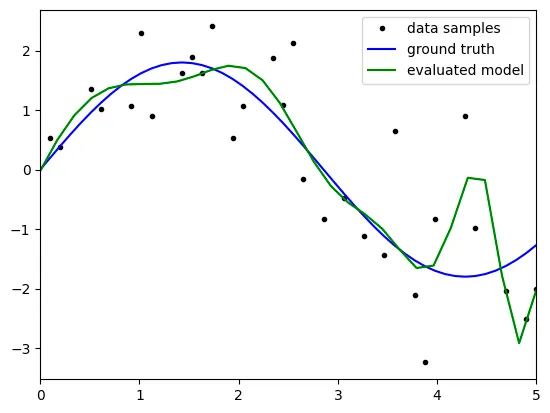
I think this curve has a good ability of unseen test samples
more than the polynomial regression with high degree
But even though the test set for this model contains many noised test set,
I think the model results well.
comparing with the polynomial regression, transforming to high degree space
with gaussian function is more independent, because there are more rooms
that we can change, which are the parameters of gaussian function.
Plain Text
복사
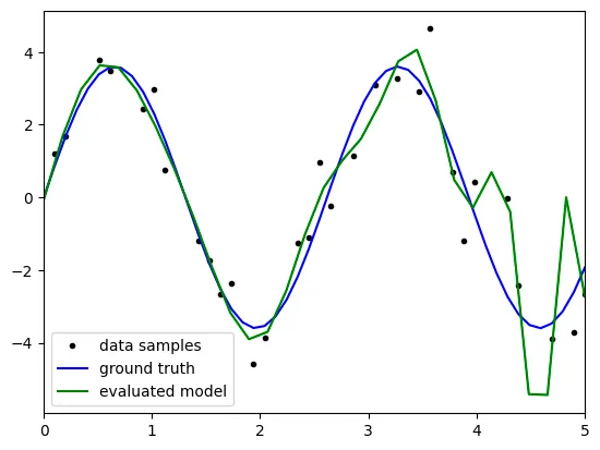
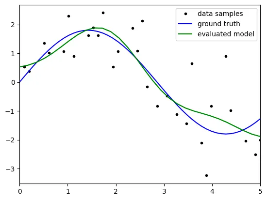
degree: 20
degree: 20
using polynomial regression with same data
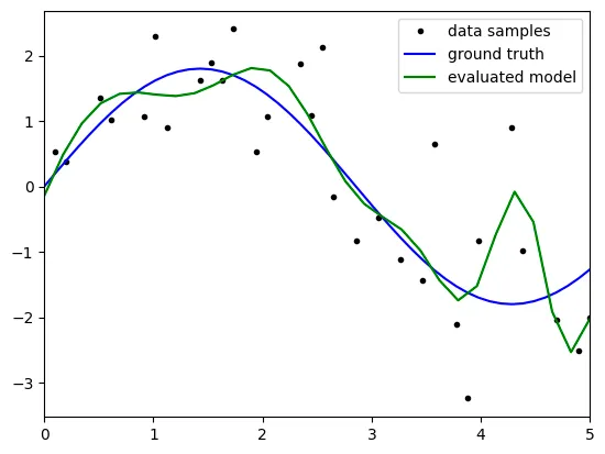
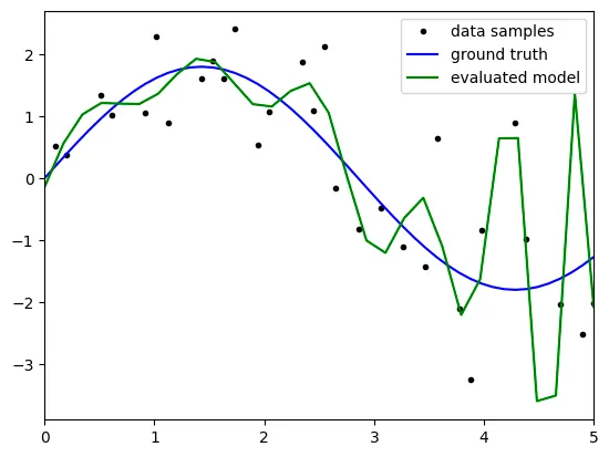
Comparing with polynomial regression, gaussian regression show less overfitting
because in the polynomial regression, the ith term goes really big.
For example, when the input is 5 and the degree is 20, the 20th term is w_20*5^20
therefore, when fitting the weight, it has bee affected by the high degree term.
However, in gaussian regression, there's no case like that.
all term is in 1 because, the distribution is 1.
Therefore, without any regularization, the gaussian basis function has
the same effect with regularization.
Plain Text
복사
Step 3: Linear Regression with Regularization
it is same as fit_gaussian function above.
there is no difference with fit_gaussian because the only difference is that there is the regressor on model.
Result
lambda: 3
lambda: 5

lambda: 10
lambda: 1
Step 4: Compute integrated squared bias and integrated variance
Result
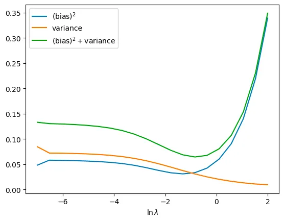
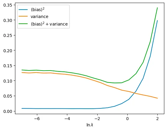
Q. Write the relationship between lambda and bias, variance.
•
when the lambda gets bigger, the variance gets smaller. However the bias gets bigger
Q. Find the best lambda value through the resulting plot and explain about it.
•
we define the error as (bias)^2 + variance.
•
Therefore we can find the beset lamda such that the ln(lambda) is about -1. then the lambda is about 1/e
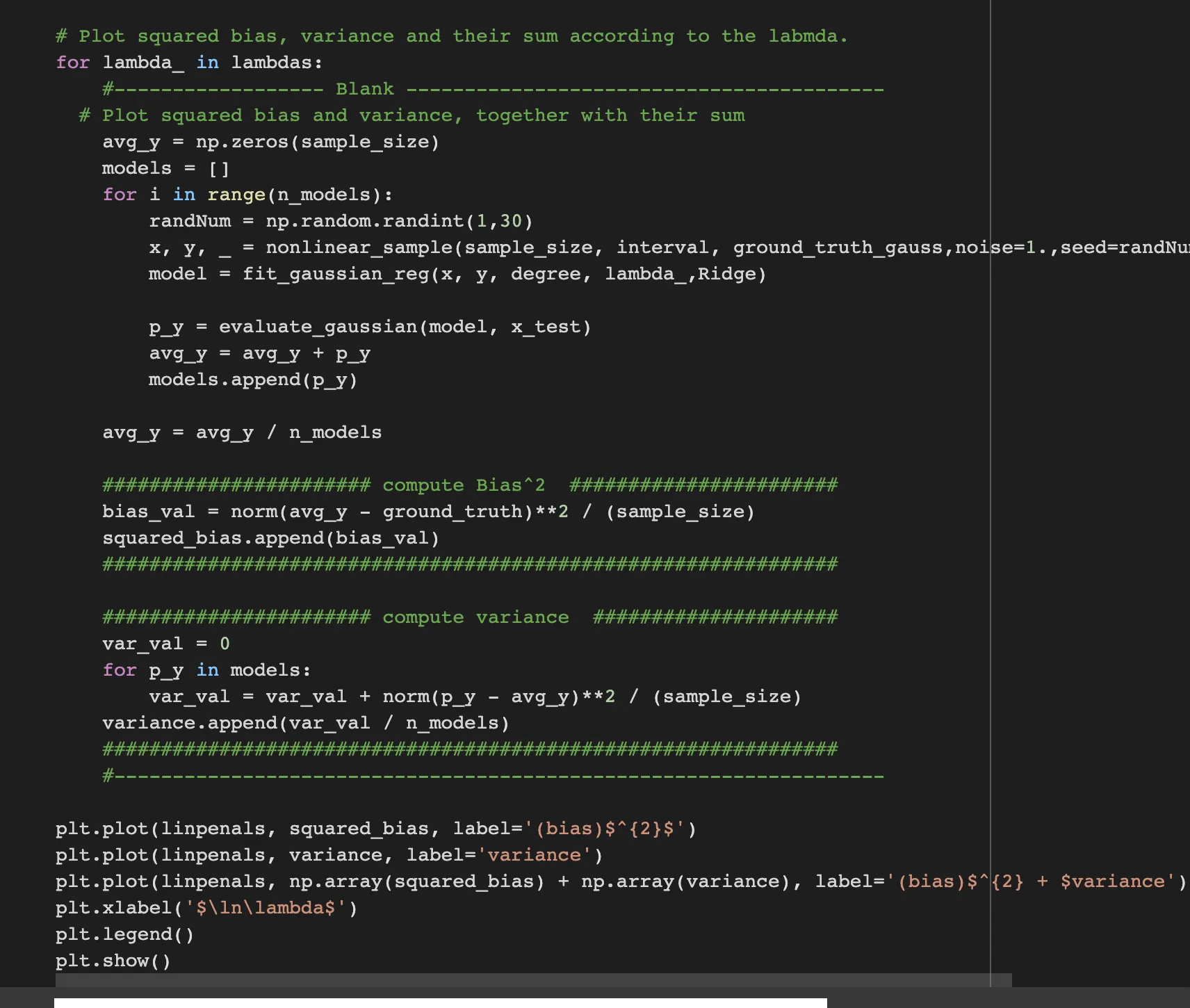
Step 5: Repeat step 4 with My_Ridge class
My_Ridge has two methods: fit and predict.
The fit method takes in input samples x and y, a learning rate lr, and the number of iterations n_iters. It initializes the weights of the model using a random normal distribution.
Then, it uses gradient descent to update the weights iteratively.
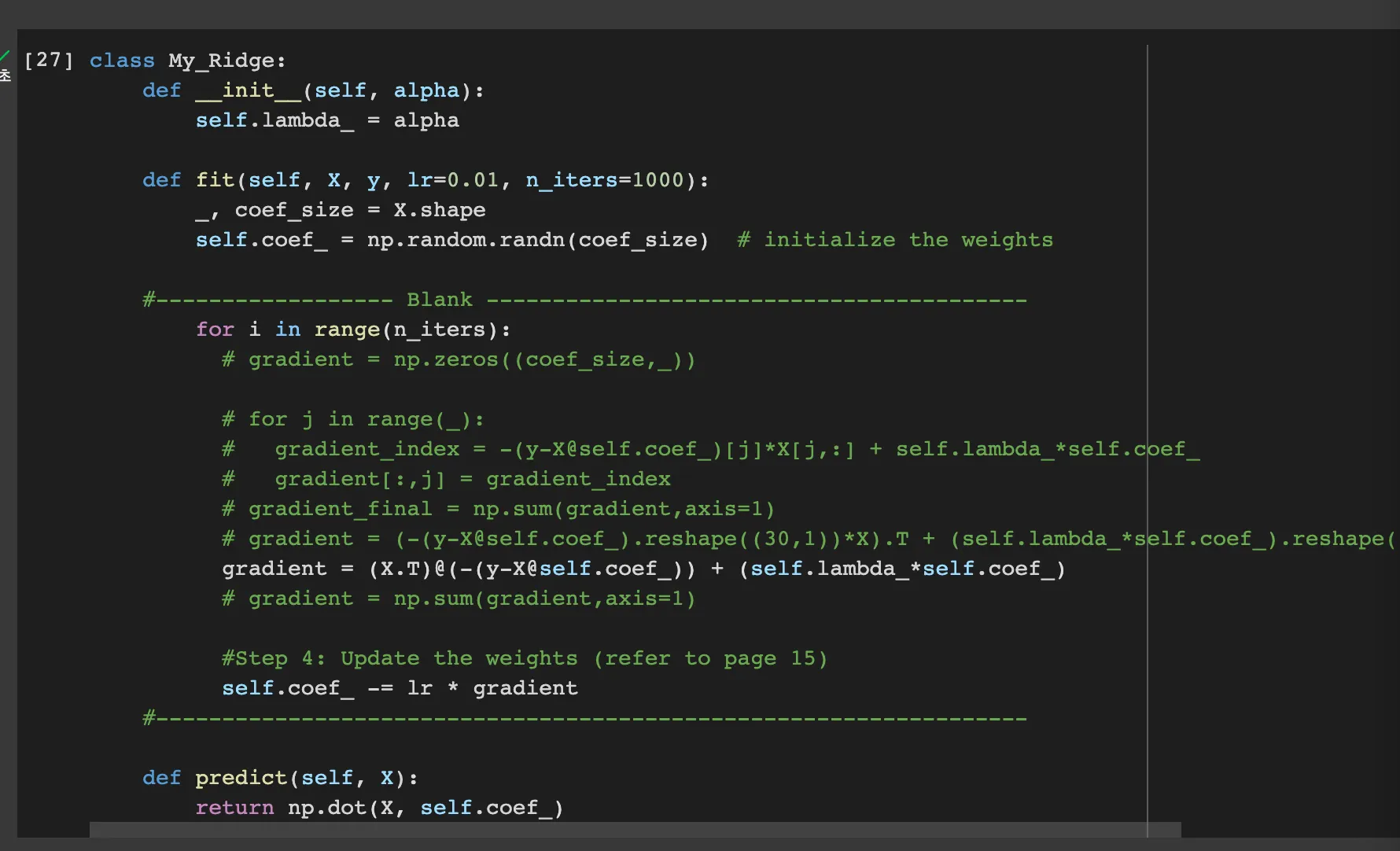
As the Ridge’s loss function is defined as
And the graident descend by w is below.
which is X is (30,6), W is ( 6,1).
which is presented as
gradient = (X.T)@(-(y-X@self.coef_)) + (self.lambda_*self.coef_)
Python
복사

for every lambda, we iterate n_models to generate models with n models.
to generate n models we’d like to generate every different sample. therefore, I decided to pass the seed number into nonlinear_sample for every iteration over n_models.
After that we compute bias and variance for each lambda.
Result
Q. Find the best lambda value through the resulting plot and explain about it.
As we defined the total error as (bias)^2 + variance, the best lambda is near the 1/e such that ln(lambda) is about -1
bigger lambda leads the bias bigger and variance smaller. Because as the regularization make the effect of the higher degree small, it leads the prediction smiliar as linear.
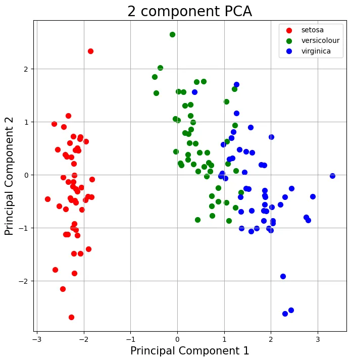
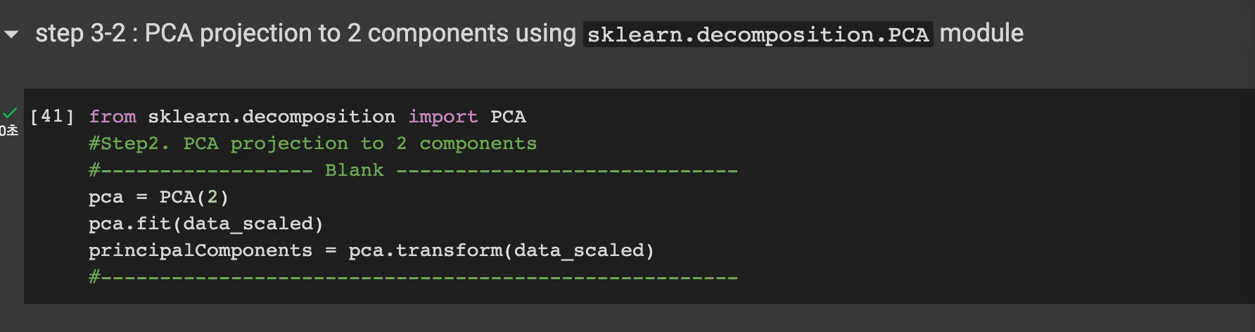
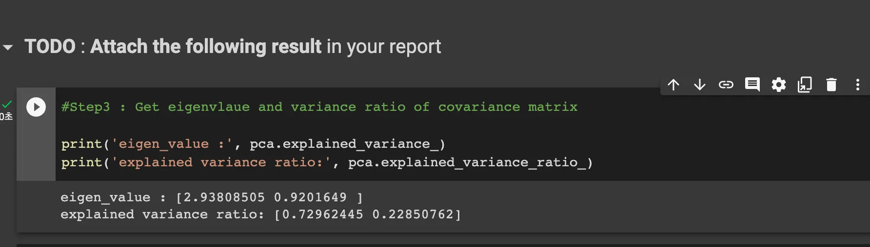
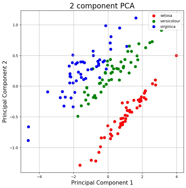
Part2: PCA
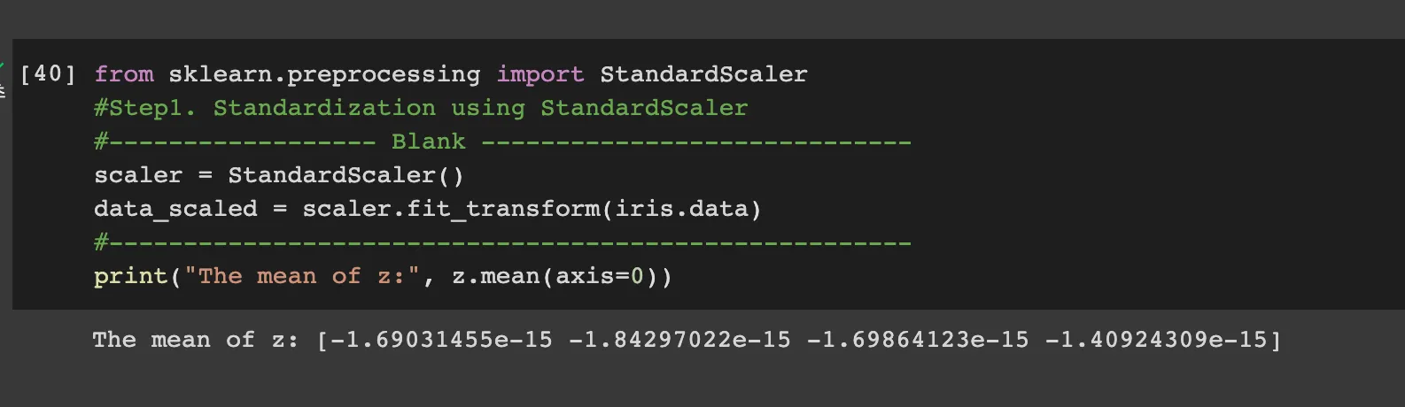
Step2-1: Standardize the dataset
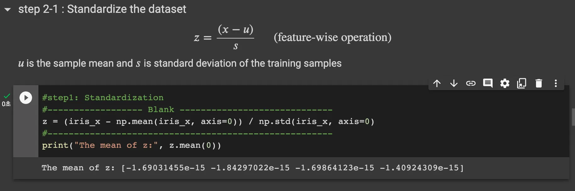
standardazation follow above equation. Therefore code is like
z = (iris_x - np.mean(iris_x,axis=0))/np.std(iris_x, axis=0)
Python
복사
Step2-4: get eigenvectors of 2 biggest eigenvalues
covariance matrix is below
Threrefore, code is like below
covar_matrix = 1/(n-1) * np.dot(z.T, z)
Python
복사
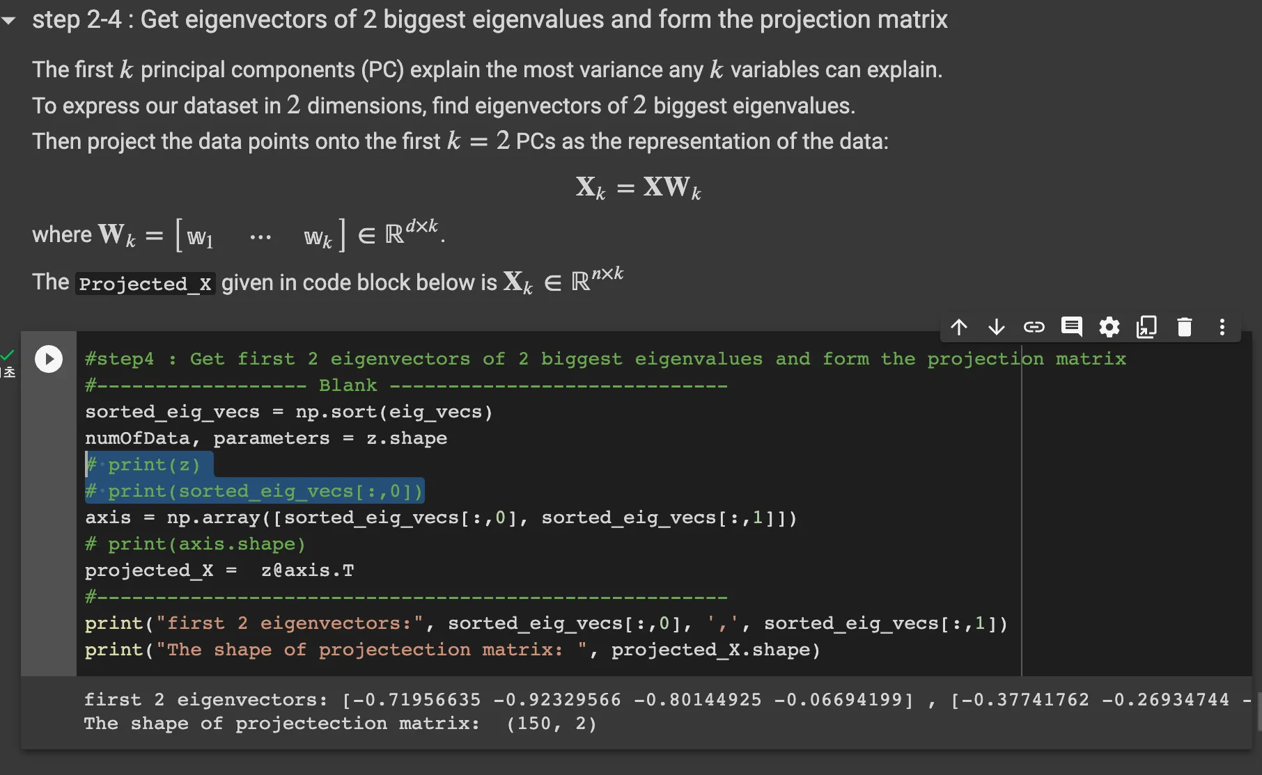
Step 2-4: Get eigenvectors of 2 biggest eigenvalues and from the projection matrix
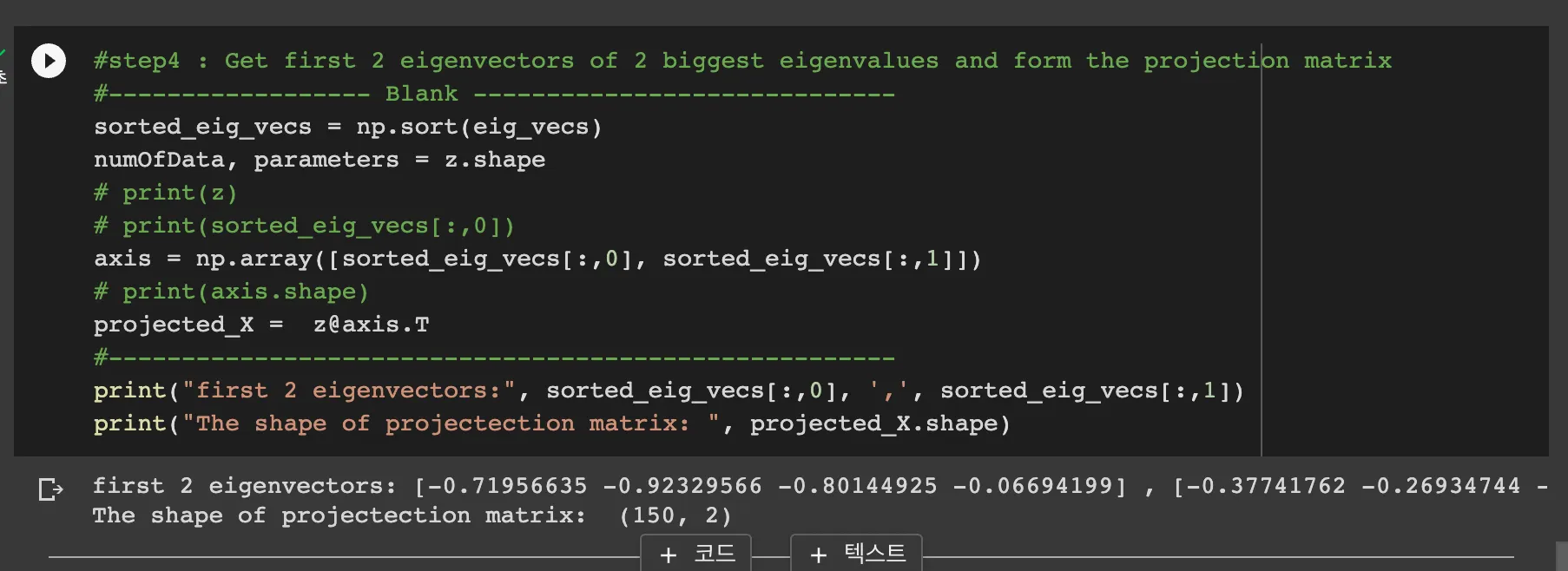
this code sorts the eig_vecs array and the axis are the 2 biggest eig_vectors.
as the projected_X is X_k = XW_k, we can do matrix operation with z and axis.T
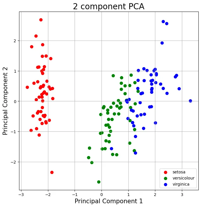
Result
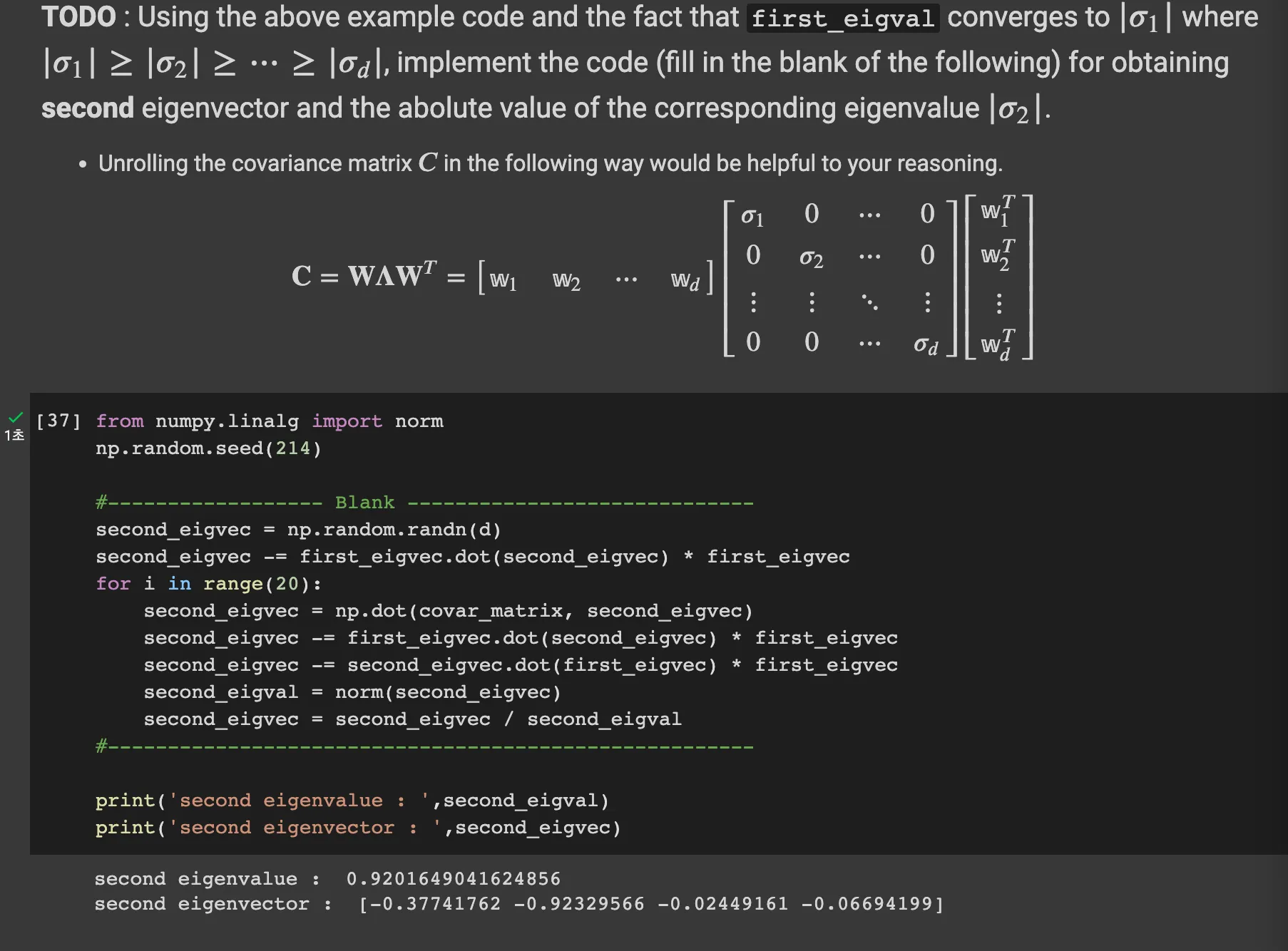
Step 2-6: get eigenvectors and eigenvalues without using np.linalg.eig()
Q. Think about the reason why above algorithm works
when the matrix is symmetric, the eigenvectors of it are always orthogonoal.
Then in the nth degree space, if there are n eigenvectors, these might be basis of the vector space. Therefore, any arbitrary vector X can be represented lineary with the basis.
As the k go big, all other terms are eliminated and only one term (Beta_1 * lambda_1^k * v1 only survives.Therefore when we divide, the norm of (A^kX) and goes infinity, the only first eigenvectors survives.
Second eigenvectors
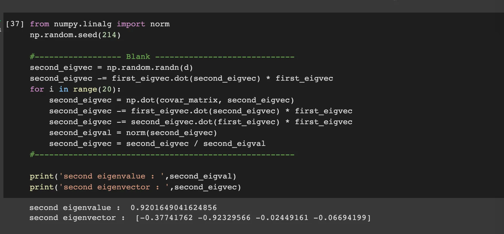
if we eliminate the term with first eigenvectors from the random vector X, then the second eigenvector is the biggest eigenvector of n-1 dimension.
Therefore we can do same power method algorithm on that.