20180036 권혁태
Part1. Implement K-means & DBSCAN
Part1-1. Implement K-means
•
fit(self,X):
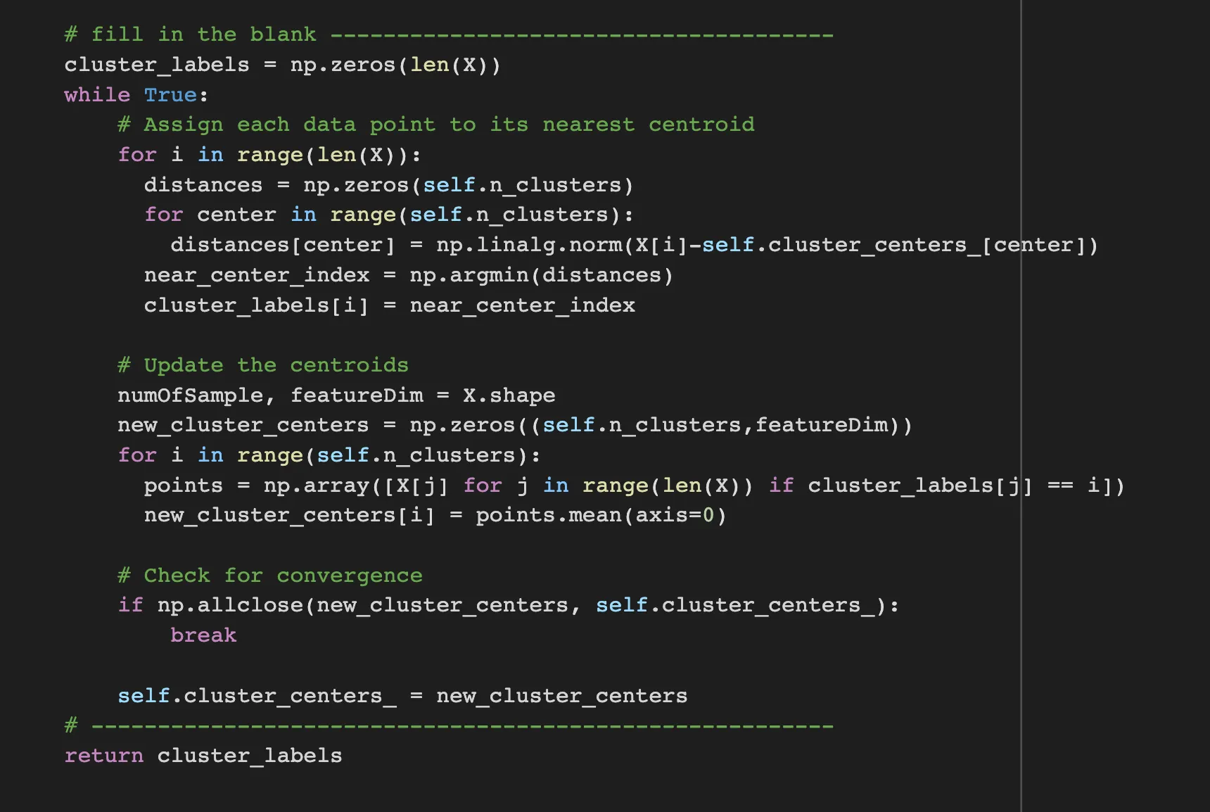
the fit(self,X) function is for calculating the distance between the centroids and points and update the positions of centroids. It constructs with 3 steps.
First step is assign the points with nearest centroids. when looping all the points, calculate the distance with centroids, and pick the nearest centroids and assign it.
Second step is drawing the center position of centroids. when looping all clusters, find the points that is assigned with the cluster’s label and get the average of all points.
And finally, check whether there is difference with the new centroids and old centroids.
•
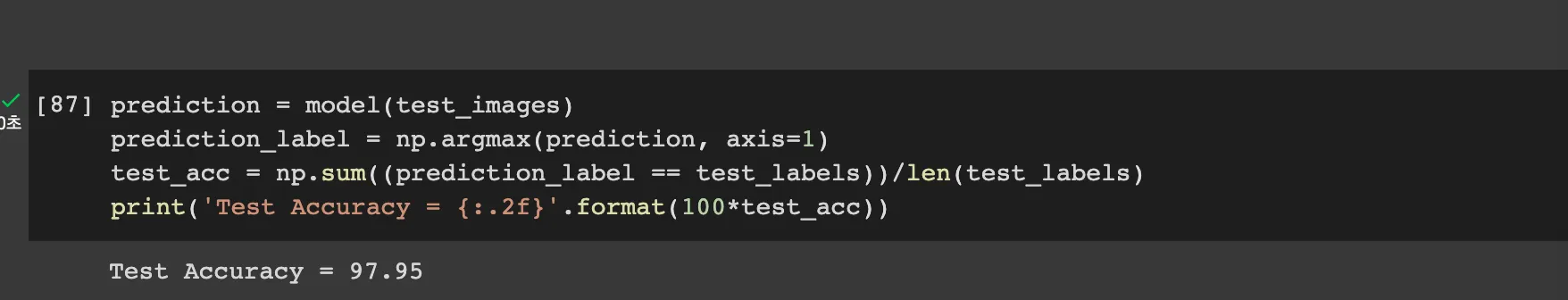
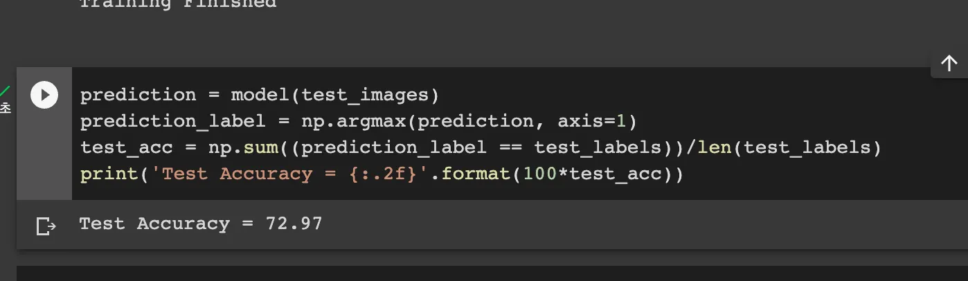
predict(self,X):
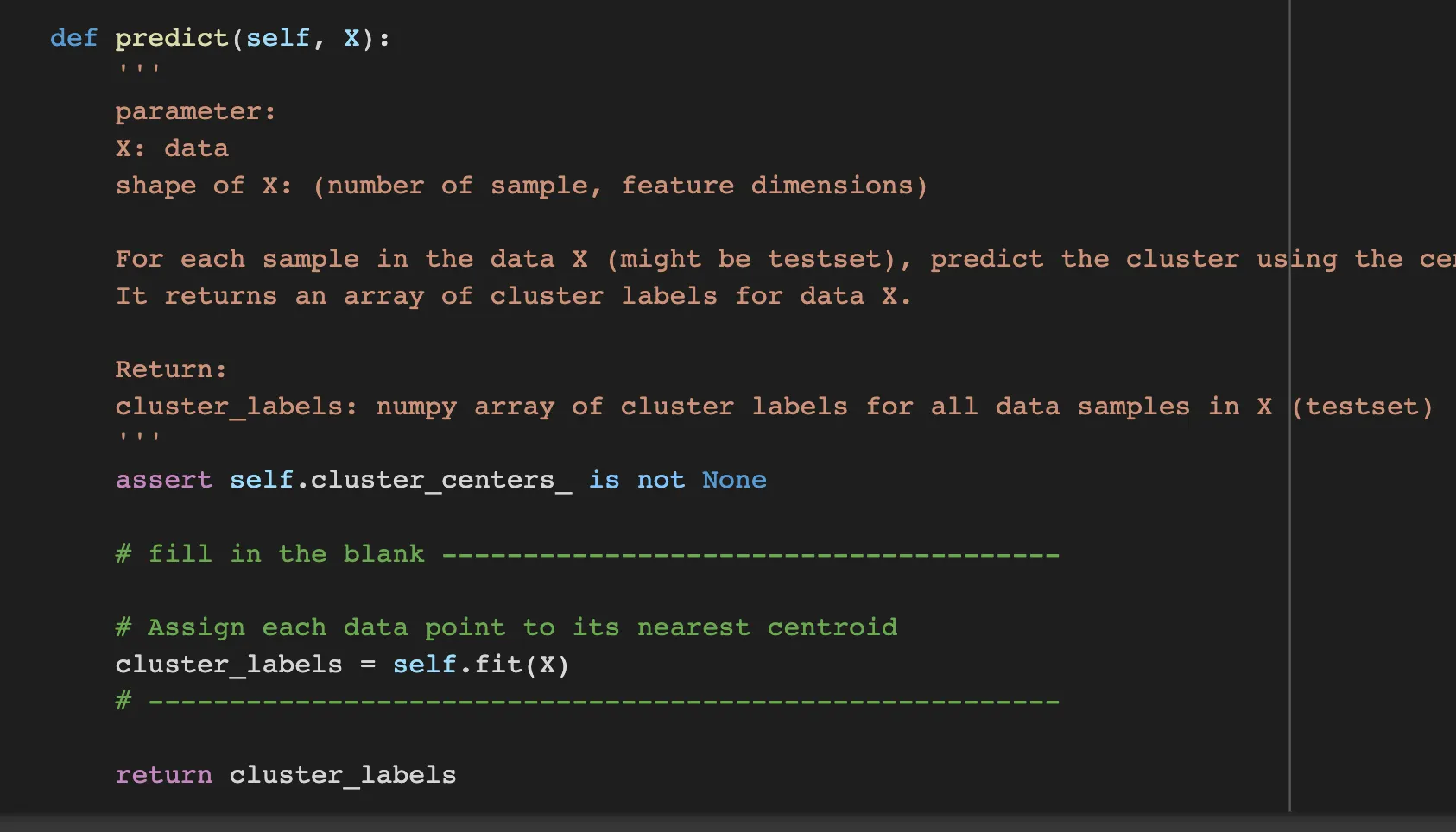
predict is so simple such that it gets the data and call fit(self,X) and return the result;
Test Result

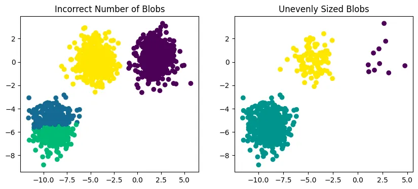
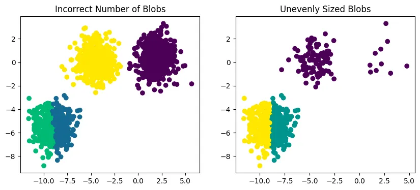
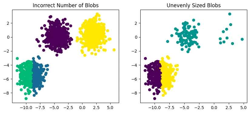
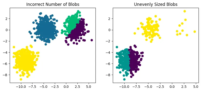
Q: various random_state Values
random_state = 500
random_state = 100
random_state = 200
random_state = 300
random_state = 400
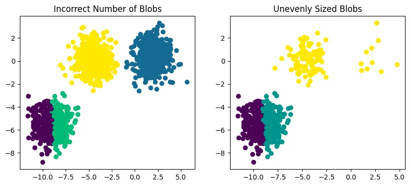
random.seed determines the random sequence from random function. Therefore, by random.seed the initial centroid points among the all points is different and this leads that the result is different for every time. this means that K-means algorithm is influenced by the initial centroid positions.
Part 1-2. Implement DBSCAN Algorithm
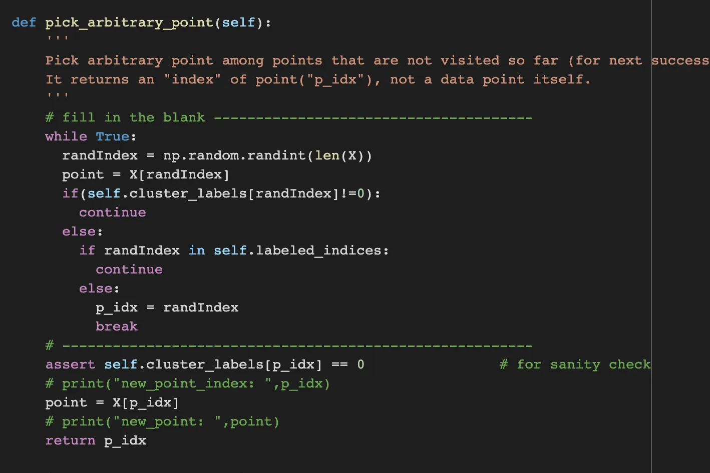
pick_arbitrary_point picks arbitrary points that is not ye marked with any clusters.
So through while statement, get a point with randomIndex and check whether it is already labeled or not.
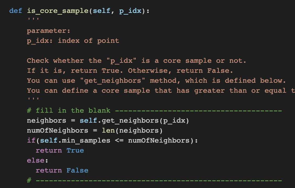
is_core_sample determines whether the point is core or not.
it uses get_neighbors such that get all neighbors within certain distance.
Therefore, we can just judge the point is core or not by checking the number of neighbors is bigger than the min_samples
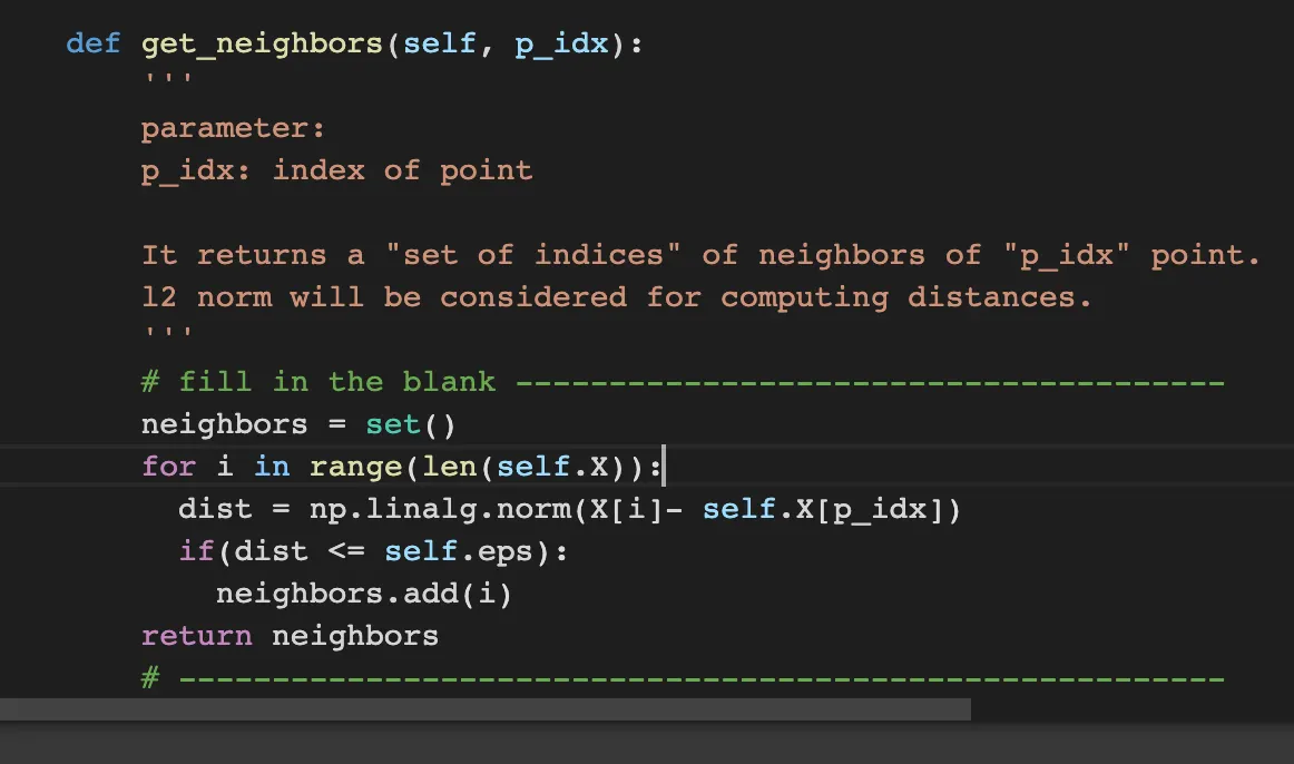
get_neighbors get all neighbors for certain point. we can get the neighbors by iterating all X and judge that the distance is less or equal than the eps.
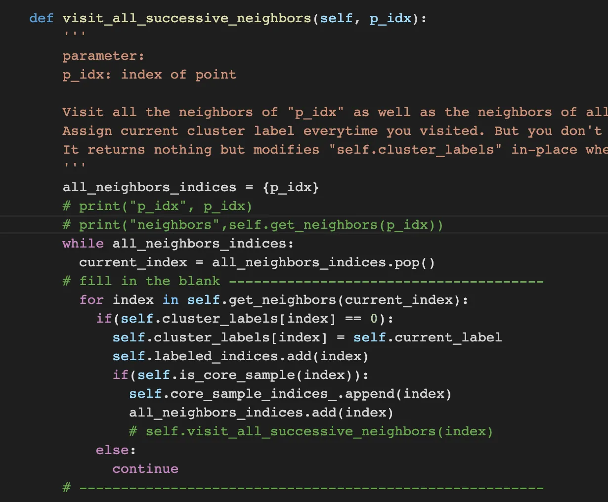
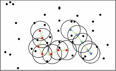
visit_all_successive_neighbors is the key of this process. this logic is kind of like BFS algorithm. First get all neighbors of certain point and add it to set. through While loop, popping from the set and get all neighbors and looping all neighbors with judge it is core_sample.
Test Results
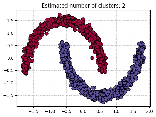
eps = 0.5, min_samples = 5
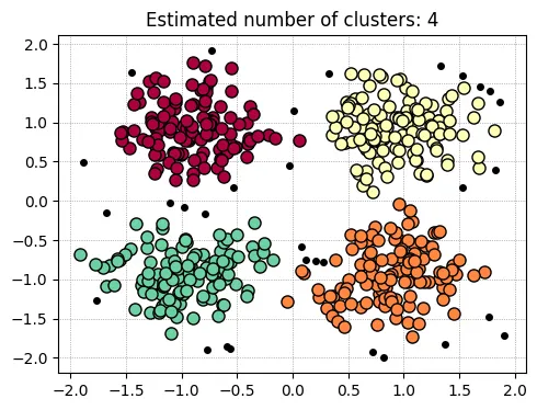
eps = 0.3, min_samples = 10
Q1. What is the main difference between noise and border point
Both point cannot be the core point by itself because they don’t have sufficient point in the range of distance. However, the difference is that the border point is labeled by the other core point but the noise is not. it means that, by the core point, the border point is labeled but the noise has no core point in their neighbors.
Q2. the clustering results are deterministic?
I think the clustering results are not deterministic because in the lecture note, there is a case that might be clustered differently depending on the order of blue point or red point.
Therefore I finally found the value.
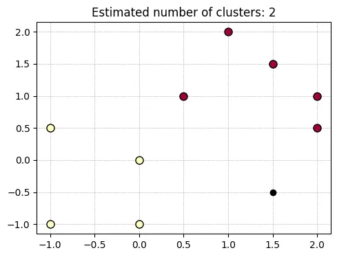
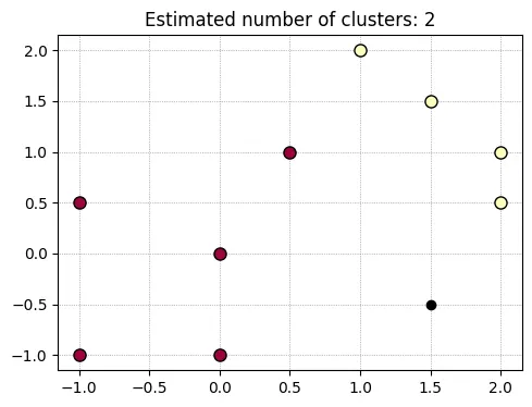
The point on (0.5, 1.0) is clustered differently depending on the visiting order. And the eps is 1.45 and min_samples are 5
Q3. Slightly modify algorithm and what is the possible range of number of noise samples after the clustering is completed.
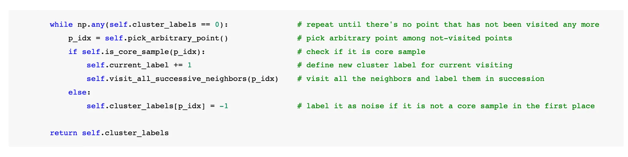
With my inferencing, the upper code just add the point which is not core point into cluster_label array. It is same as not determining the point, just holding the state as ‘not classified’. Therefore, there can be room such that the not-core point can be labeld by as border point of other core point.
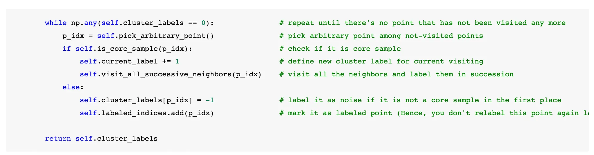
However, the second code just determines whether the point is noise or not. However, the point is arbitrary picked and judge the point by just away, even the point can’t be real noise point, it can be judged as noise point.
In short, the core point is not different with two codes because the core point is always core point regardless of determining as noise point earlier or not.
However, the noise point, especially the max number of noise point will increase when using second codes. Let’s assume following situation such that for every each arbitrary point, if the point is not core. Then all the point we pick is all noise. Therefore the number of max noise m is just total number N subtracted by the core points C. (m = N - C)
with first codes, as it allows the chance that the not-core point can be classified as border point by other core points, the max number of noise is less than the case using second codes.
Part2. Numpy Implementation of autograd, torch-like Tensor and Module
Task1. Implement backward of the operations
Add
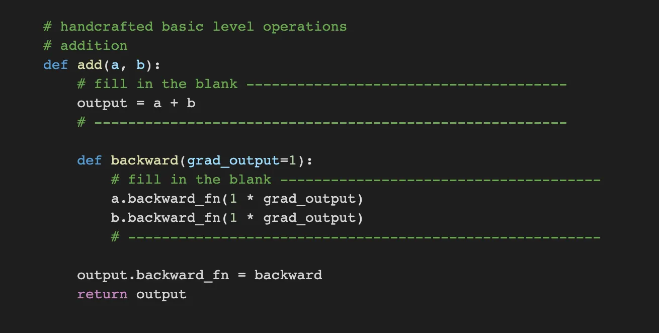
Add is just adding the numbers. Therefore, output is adding the numbers. And backward for adding is just one because the differential of a+b by a is just one
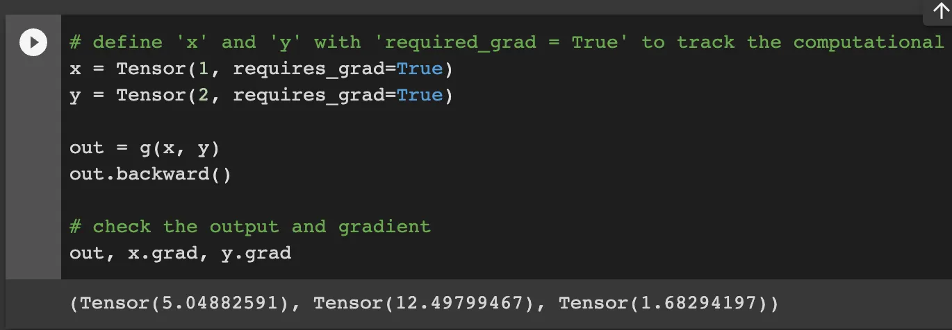
Multiply
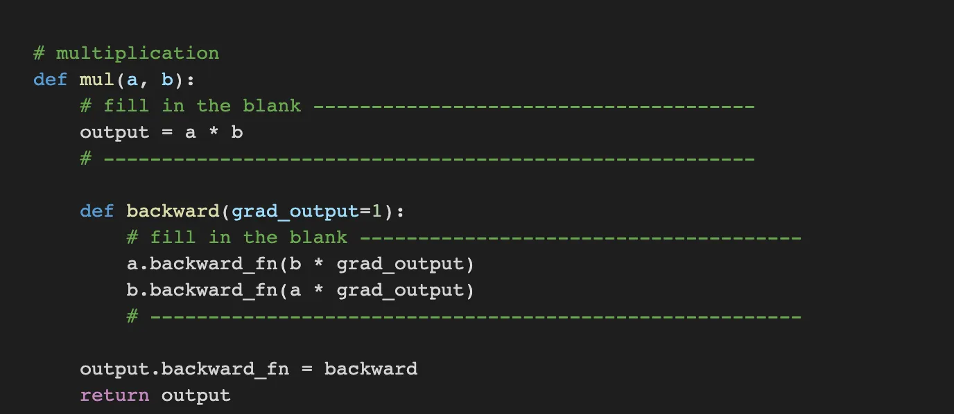
Mul is just multiplying the numbers. Therefore, output is multiplying the numbers. And backward for multiplying is the other element because the differential of a*b by a is b.
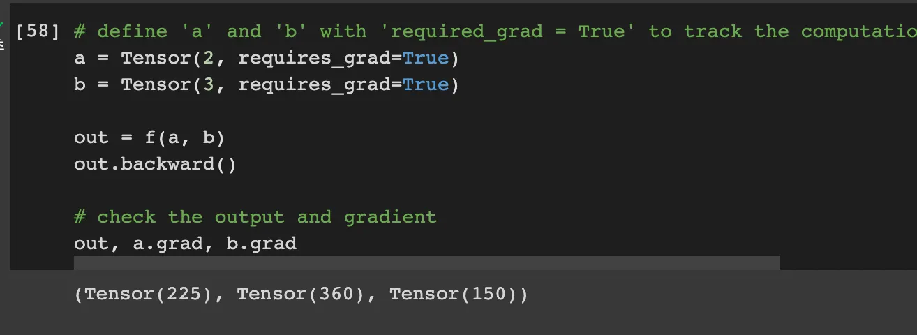
Result
sin
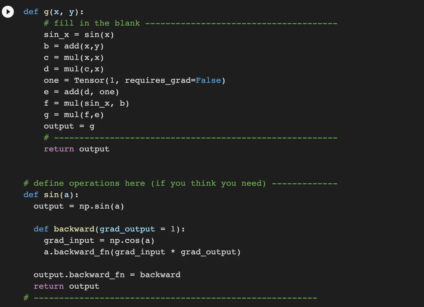
sin must be defined for backward like add and multiply. Because the sin takes one parameter, we can define sin with one parameter. And it’s backward is cos so that we can process backward process with cos * grad_output
Result
Task2. Implement zero_grad() and update() methods
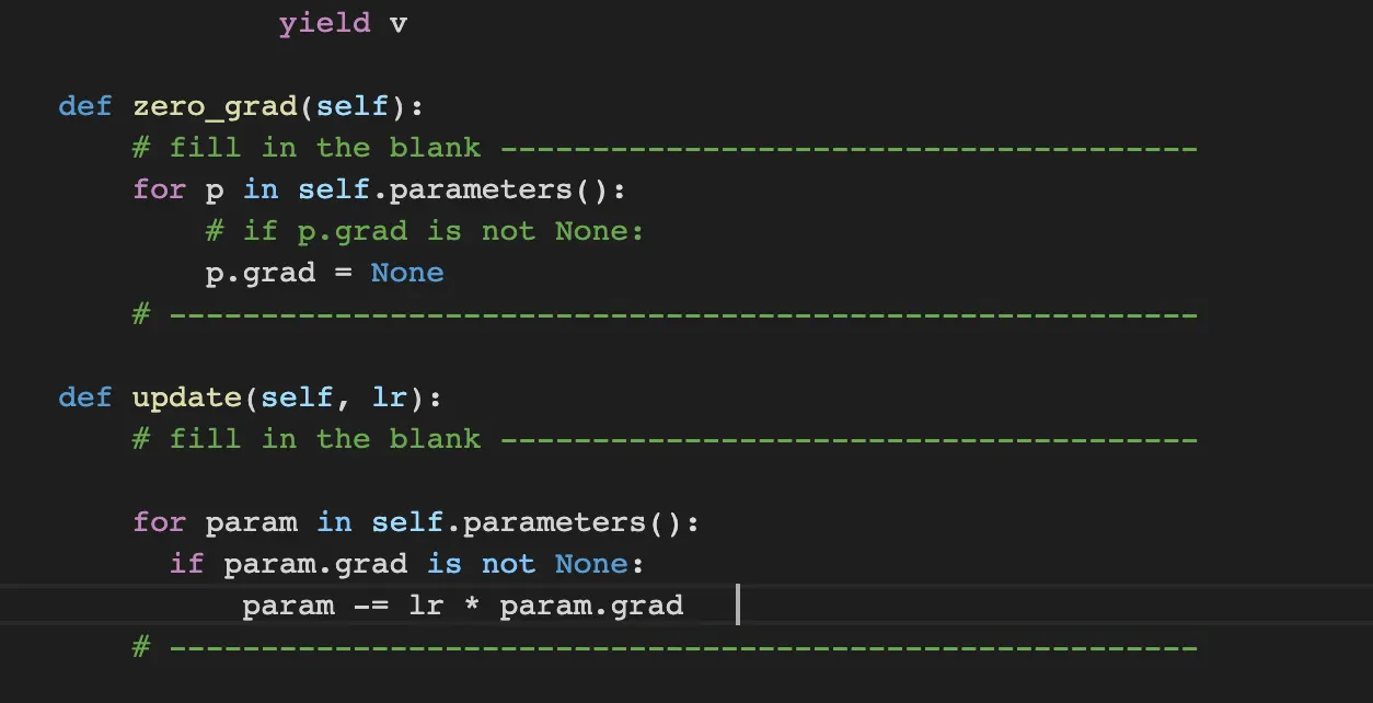
zero_grad makes all parameter’s gradient makes zero. Therefore, I iterate all parameters with self.parameters() and make the grad of the param to zero.
update changes the parameter’s gradient with learning rate and current gradient. Through this method, the gradient of parameters are optimized.
Result
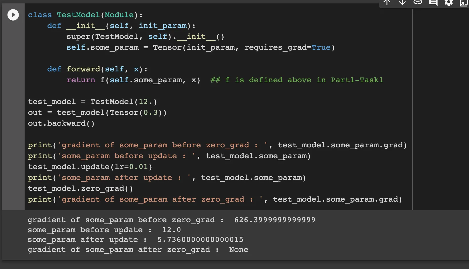
Through TestModel, we can figure out that the gradient descent is well done.
Task3. Implement ReLU, Linear Modules
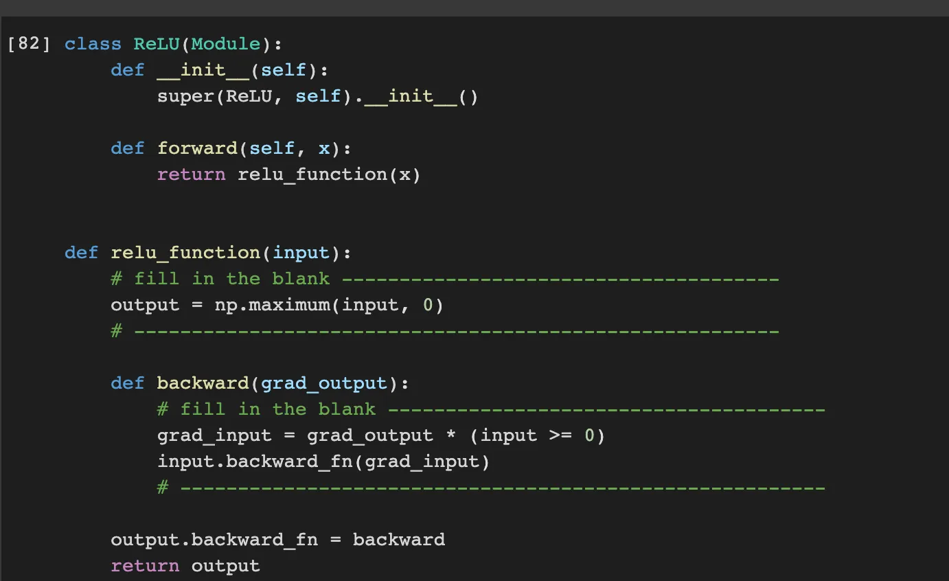
ReLU is the function which results same as input when the input is greater or equal than zero.
Therefore the output is np.maximum(input, 0). Also when backward propagation, grad_input which will passed to former layer is same as grad_output which is passed from the next layer.
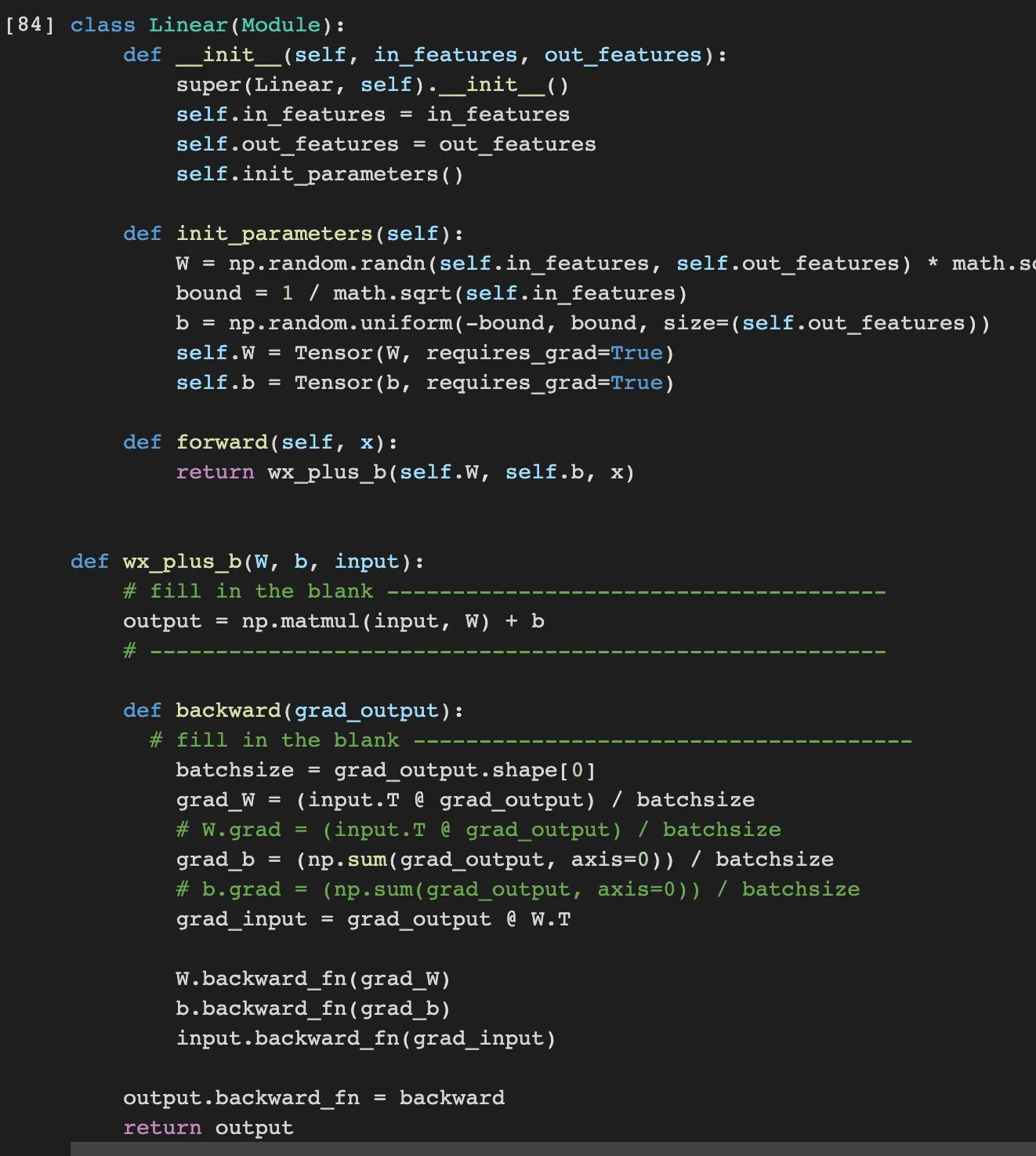
Linear is the element wise multiplication with W and input and adding bias. Therefore the output in forward process is np.matmul(input,W) + b
When doing backward propagation, the differential of output on input is just W. Therefore the the gradient passed to former layer is just multiply the grad_output which is passed from next layer and W.T
Also, we should call backward_fn of W and b so that the gradient of it is updated.
Task4. Implement CrossEntropyLoss
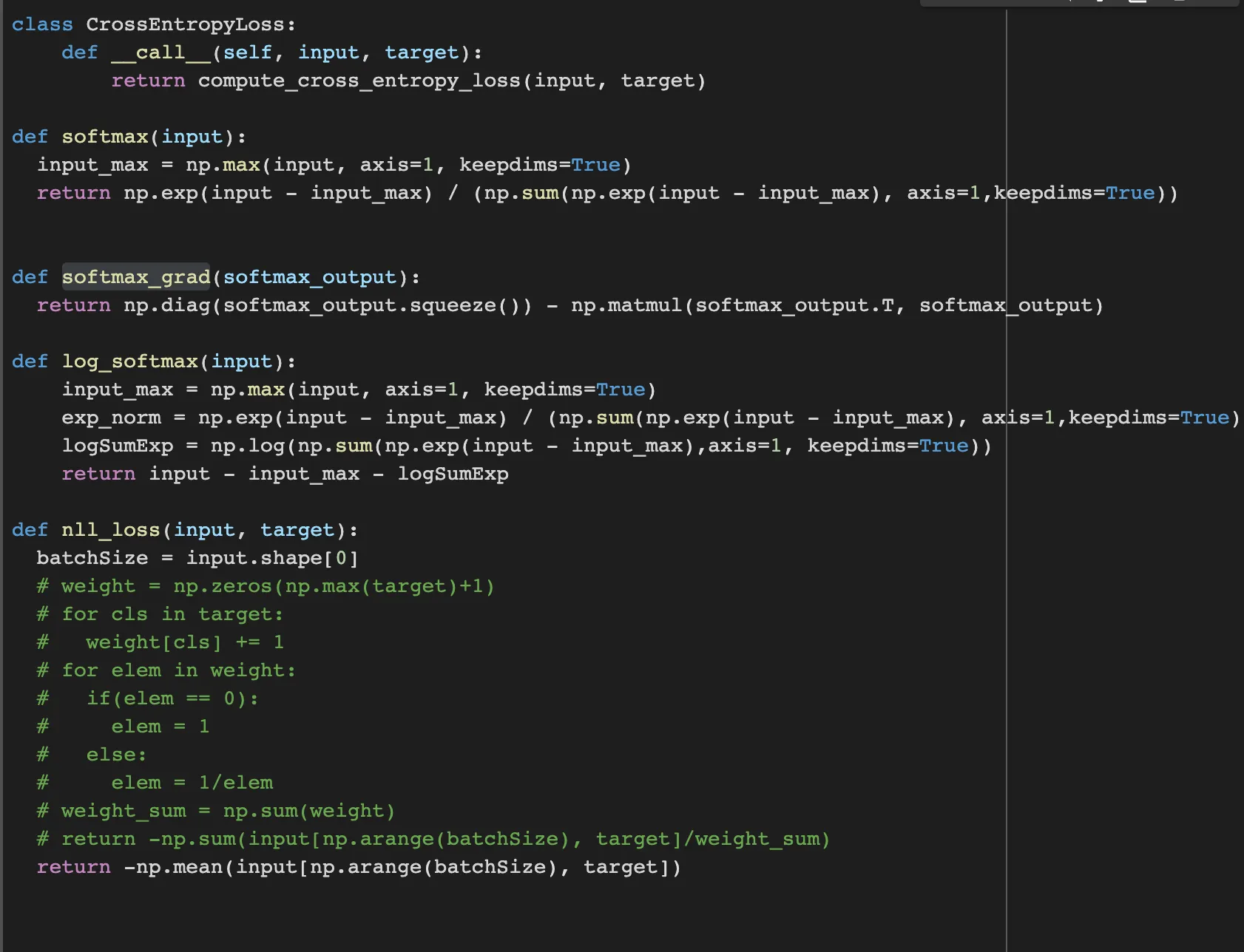
CrossEntropyLoss is used to compute the cross-entropy loss between the input and target.
The softmax function computes the softmax activation function. It first normalizes the input by subtracting the maximum value in the exponents. And it normalized input by dividing the sum of exponentiated normalized inputs.
The softmax_grad function takes the output of the softmax function as input and returns the gradient of the softmax function with respect to its input.
The log_softmax function computes the log-softmax activation function.
It first normalizes as same as softmax function. However, the only difference is that, It takes the logarithm of the output of softmax function.
The nll_loss function computes the negative log-likelihood loss between the input and target.
I’m just getting the proper probability with target array by indexing from input and get the mean value of all loss. I also implement with weights, which introduced in pytorch document, but there is no standing difference in accuracy, so I remove it.
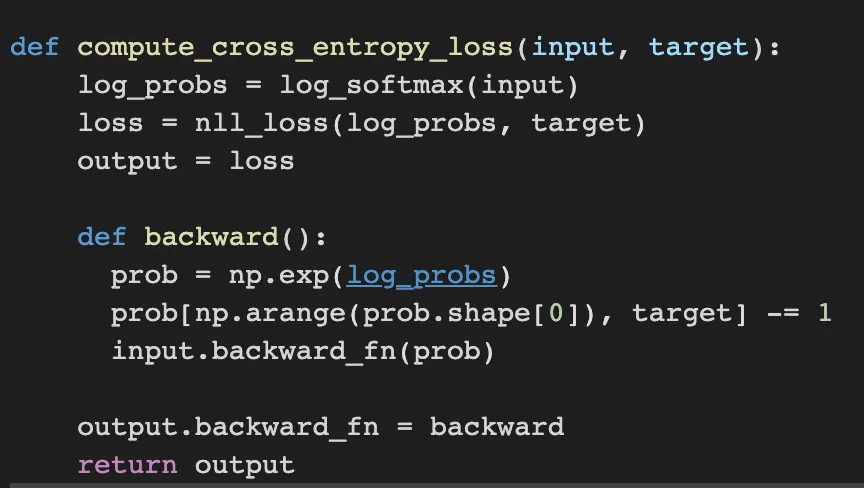
The compute_cross_entropy_loss function computes the total loss through log_softmax and nll_loss.
The backward function get the gradient of loss and it pass to former layer. the gradient of cross_entropy_loss is just difference with target and probability so I can just subtract 1 on the probability.